From Photons to Electron Counts
Chapter 1 established what sampling means mathematically. This chapter asks: what does the hardware physically do at each sample point? The answer involves photons, quantum mechanics, and irreducible randomness.
12.1 The Photosite
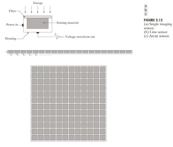
A camera sensor is a grid of photosites — tiny light-sensitive elements, one per pixel. Each photosite executes the sampling operation from Chapter 1 at its spatial location. During the exposure time it:
Collects photons arriving from the focused scene
Converts photons to electrons via the photoelectric effect (one photon → at most one electron)
Accumulates electrons in a potential well until readout
Reads out the charge as a voltage, then converts it to a digital integer via an ADC
The integer that emerges is the pixel value. It is a count of electrons — a proxy for the number of photons that arrived, which is itself a proxy for scene brightness.
22.2 Photon Counting Is Inherently Random
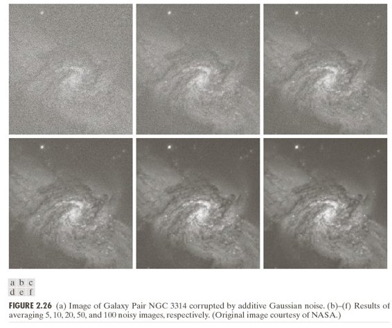
Photon arrivals are a Poisson process: independent random events occurring at some average rate (photons per second per photosite area). Even if the scene is perfectly uniform and the sensor is perfect, the count in any one exposure is random.
For a Poisson process with mean :
The standard deviation equals the square root of the mean. This is shot noise — not an instrument defect, but a fundamental consequence of the discrete nature of light.
Implication: even a perfectly flat, perfectly lit, perfectly uniform scene produces pixel values that vary from photosite to photosite. The variation scales as .
32.3 Signal-to-Noise Ratio
Signal is the mean electron count . Noise has two contributions:
Shot noise: — from photon statistics
Read noise: — from the amplifier and ADC circuitry
Total noise in quadrature:
At high signal () this simplifies to:
Doubling the signal improves SNR by .
42.4 Key Sensor Parameters
| Parameter | Symbol | Typical phone | Typical DSLR | Effect |
|---|---|---|---|---|
| Photosite area | ~1 µm² | ~25 µm² | Larger → more photons → higher SNR | |
| Full-well capacity | ~1,000 e⁻ | ~50,000 e⁻ | Maximum before saturation | |
| Read noise | ~3 e⁻ | ~5 e⁻ | Noise floor | |
| Quantum efficiency | QE | 0.4–0.6 | 0.5–0.8 | Fraction of photons → electrons |
Mean electron signal: where is photon flux and is exposure time.
52.5 Phone vs DSLR — Why Sensor Size Matters
A DSLR photosite is roughly 25× larger than a phone photosite. Same scene, same exposure time → DSLR collects 25× more photons → .
This is not about optics quality or processing — it is pure geometry. A larger bucket catches more rain.
| Condition | Phone | DSLR |
|---|---|---|
| Bright daylight | Good | Good |
| Indoor | Noisy | Acceptable |
| Night | Very noisy (SNR ≈ 1) | Usable |
Critical consequence for computer vision: pixel values from a phone and a DSLR of the same scene are not numerically comparable, even at the same exposure settings. The pixel value encodes sensor physics, not just scene brightness.
62.6 The Pixel Value Equation
where is the ADC mapping and is dark current noise. Every term except (photon flux from the scene) is a camera-specific nuisance. Two cameras imaging the same scene produce different pixel values — not because the scene differs, but because their hardware parameters differ.
This is the root of the problem explored in Chapter 6.
Run:
uv run python tutorials/00_introduction_to_digital_images/part2_sensor_physics.pyto generate SNR vs brightness curves and the shot noise simulation.
7Summary
| Concept | Key fact |
|---|---|
| Photosite | Converts photons to electrons; one per pixel |
| Shot noise | — irreducible, from photon statistics |
| SNR | at high signal; bigger photosite = higher SNR |
| Full-well capacity | Max electrons before saturation = white clipping |
| Pixel value | Encodes scene brightness + sensor physics + noise |
Next → Chapter 3 — Pixels: the sensor produces a grid of integers — what does that grid mean, and what are its limits?