11. The Clean World¶
Forget models for a moment. You are an engineer with a sensor.
You have a source — some thing in the world with a value you want to measure. A temperature. A distance. A concentration. A pixel intensity at a particular location on a scene.
You point a sensor at it and read out a number — the measurement.
If the sensor were perfect, the measurement would equal the true value exactly.
Formally: we have an input (what we control, or what identifies the source) and a measurement we read off the sensor. There is some relationship
where is whatever the underlying physics dictates — linear, exponential, wavy, arbitrary.
Two examples to fix the idea:
| (source) | (measurement) | ||
|---|---|---|---|
| Thermometer | True room temperature | Linear scaling (sensor response) | Reading on the display |
| Camera pixel | Light hitting the surface (scene radiance) | Lens + sensor transfer function | Gray-level pixel value |
In both cases, a perfect sensor would give you exactly — no guesswork, no error. The thermometer would read the true temperature; the pixel would perfectly encode the true brightness.
In a perfect world, machine learning wouldn’t exist. If you knew , you’d just plug in and read off . No learning, no estimation, no uncertainty. The entire ML and signal-processing industry hinges on everything that comes next.
import numpy as np
import matplotlib.pyplot as plt

x_grid = np.linspace(0, 10, 200)
true_f = lambda x: 2.0 * x + 0.5      # perfect linear sensor
y_clean = true_f(x_grid)

fig, ax = plt.subplots(figsize=(8, 4.5))
ax.plot(x_grid, y_clean, linewidth=2.5, label='y = f(x) (the truth)')
ax.set_xlabel('x (input / knob setting)')
ax.set_ylabel('y (sensor reading)')
ax.set_title('The clean world — perfect sensor, no ML needed')
ax.legend()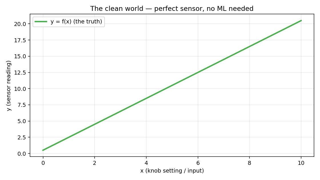
22. Modelling the World¶
Look back at what we just did. We pointed at “a thermometer in a room” and wrote . The room is not an equation. The thermometer is not an equation. We replaced a physical situation with a symbolic stand-in — a few letters and an equals sign — and then promised ourselves we’d do all our reasoning inside the symbols.
That swap has a name. It is called mathematical modelling, and it is the move that makes engineering and science possible. You cannot compute on a room. You can compute on . Every prediction ever made — by a calibration curve, by a Kalman filter, by GPT-5 — is a calculation performed inside a model and then projected back onto the world.
A worked example: a falling ball¶
Drop a ball from a height . We want to know how high it is at time . From classical mechanics, with gravity :
That single line is a model. It compresses the entire physical situation into:
A variable we control or observe: (time since release).
A variable we want to predict: (height).
Parameters: (release height) and (gravitational acceleration).
A functional form: a downward parabola.
import numpy as np
import matplotlib.pyplot as plt

g = 9.81                                  # m/s^2
h0 = 10.0                                 # release height in metres
t = np.linspace(0, np.sqrt(2 * h0 / g), 200)
h = h0 - 0.5 * g * t**2

fig, ax = plt.subplots(figsize=(7, 4))
ax.plot(t, h, linewidth=2.5)
ax.set_xlabel('time t (seconds)')
ax.set_ylabel('height h (metres)')
ax.set_title('A model of a falling ball: h(t) = h₀ − ½ g t²')
ax.grid(True, alpha=0.3)
What does the model give you?
Predictions at unseen . You never measured , but the model tells you the ball is at metres. This is the whole point: a model lets a finite act of understanding cover infinite cases.
A place to plug data in. If you don’t know exactly, you can measure a few heights at known times and fit to the data. The model has turned a physics question into an arithmetic one.
A vocabulary for arguing. “Did the ball fall faster than expected?” is now answerable: compare measurements to and look at the residual.
What this model throws away¶
Every model is a deliberate lie. This one is missing:
Air resistance — real balls slow down; the model doesn’t.
The ball’s shape, mass, and spin — none appear in the equation.
The Earth’s curvature and the variation of with altitude — is treated as a constant.
The fact that “height” is measured relative to something — the ground, the release point, sea level — and that choice matters when you compare to data.
These omissions are not bugs. They are the model’s whole point. Including everything would give you back the world, which is precisely what you were trying to escape. The skill is throwing away the things that don’t matter for the question you’re asking.
“All models are wrong; some are useful.” — George Box
A model isn’t judged by whether it is true. It is judged by whether predictions made through it survive contact with new data.
Why this matters for the rest of the book¶
Everything in computer vision and machine learning is a model of something:
A pinhole-camera equation is a model of how light becomes pixels.
A Gaussian distribution is a model of how noise behaves.
A convolutional network is a model of how local image patterns combine into objects.
A transformer is a model of how tokens depend on each other.
You will spend the rest of the book learning which models work for which questions, and what each one quietly throws away. The clean world of §1 is the easy case where the model holds perfectly. The next section is what happens when you actually run an experiment and the model and the world stop agreeing.
33. Noise Enters¶
Real sensors don’t give you . They give you . The garbage has physical origins:
Thermal noise — electrons jiggling due to temperature; reducible by cooling but never fully eliminable.
Shot noise — photons and electrons arrive at random discrete times, not as a smooth continuous stream; present in every semiconductor device (photodiode, CMOS pixel, transistor) regardless of temperature.
Quantization — the ADC rounds to the nearest integer count.
Calibration drift — the sensor baseline changes over hours or days.
Stray light / EM interference — unintended signals leaking in.
Mechanical vibration — the source or the sensor moved slightly between readings.
You cannot predict the garbage on any particular reading. What you can predict is its statistics — its distribution, its mean (often 0), its variance.
Running the same measurement many times¶
Hold fixed. Read the sensor 1000 times. In the clean world the readings would all be identical. In reality they scatter:
x_fixed   = 5.0
true_value = true_f(x_fixed)   # = 10.5
noise_std  = 0.8
num_reads  = 1000

# Each reading = true value + independent Gaussian noise
readings = true_value + np.random.randn(num_reads) * noise_std

print(f"True value : {true_value}")
print(f"Sample mean: {readings.mean():.4f}")   # close to true_value
print(f"Sample std : {readings.std():.4f}")    # close to noise_std

fig, axes = plt.subplots(1, 2, figsize=(13, 4.5))

# Left: scatter of readings over time
axes[0].scatter(range(num_reads), readings, s=8, alpha=0.6)
axes[0].axhline(true_value, linestyle='--', label=f'true value = {true_value}')
axes[0].set_xlabel('reading number')
axes[0].set_ylabel('sensor output y')

# Right: histogram — noise has structure (bell shape)
axes[1].hist(readings, bins=40, alpha=0.7, edgecolor='white')
axes[1].axvline(true_value, linestyle='--', label='true value')
axes[1].axvline(readings.mean(), label=f'sample mean = {readings.mean():.3f}')
axes[1].set_xlabel('sensor output y')
axes[1].set_ylabel('count')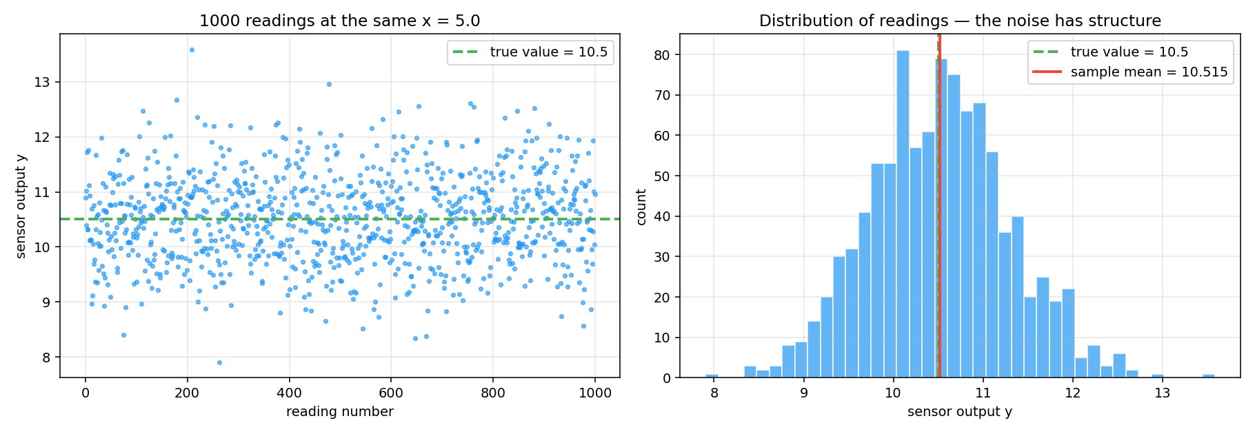
Two observations that matter for everything that follows:
Single readings are almost useless. No individual reading equals the truth. The best we can say is “probably within the typical spread of the truth.”
The readings aren’t random in a lawless way. They cluster — the distribution has a shape, a mean, a spread, symmetry. Noise is unpredictable at the level of one sample but predictable at the level of many.
That second point is the foundation of everything. We can’t beat noise on a single reading, but we can characterize it well enough to design algorithms that work on average. The mathematical name for this is statistics.
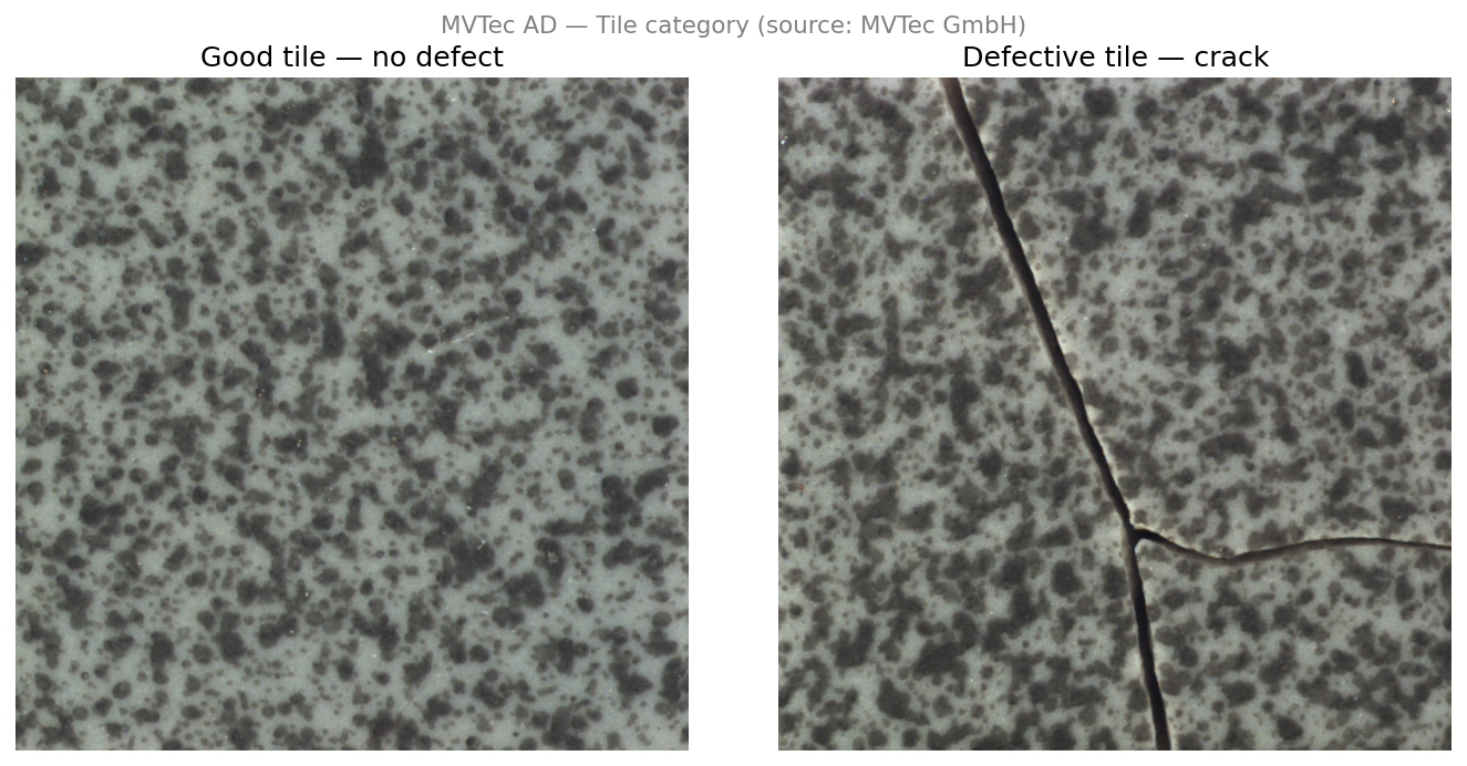
Running example — MVTec AD, Tile category
We will use one concrete dataset throughout this book to keep the abstractions grounded.
The MVTec Anomaly Detection (MVTec AD) dataset is a public industrial surface inspection benchmark from MVTec GmbH. We use the Tile category — grayscale images of ceramic tile surfaces captured under controlled overhead lighting by a monochrome camera. Some images contain defects (cracks, glue strips, discolorations, rough patches); most do not. The task: decide whether a surface patch is defective.
Abstract Concrete (MVTec Tile) Source a surface patch at a fixed location True value true surface reflectance at that patch Measurement gray-level pixel value recorded by the camera Noise sensor thermal noise, shot noise, stray light This one dataset will be attacked three ways across the book:
Attack 1 — average and filter images to suppress noise and reveal defect structure
Attack 2 — fit a parametric texture model; flag patches that deviate from the fitted surface
Attack 3 — train a CNN on labeled defect/no-defect patches
In a perfect sensor, the pixel values would encode true reflectance exactly and defects would be trivially visible. In practice, noise and texture variation make this hard — and that difficulty is exactly what drives everything that follows.
44. Why Is the Noise Gaussian?¶
Look at the histogram in §3. That bell shape isn’t coincidence. In physics and engineering, measurement noise is overwhelmingly Gaussian, and there is a deep reason: the Central Limit Theorem (CLT).
The CLT says: if you add up many independent small random contributions, each from some distribution (any distribution, as long as each has a finite variance), the sum tends to be Gaussian-distributed — regardless of the individual distributions.
Your sensor’s noise is the sum of many tiny independent contributions: thermal, quantization, vibration, EM. By the CLT, their aggregate is approximately Gaussian. This is physics, not a mathematical convenience.
num_draws = 50_000
K_values  = [1, 3, 10, 30]   # number of uniforms to sum

fig, axes = plt.subplots(1, 4, figsize=(15, 3.5))

for ax, K in zip(axes, K_values):
    # Sum K independent uniform(-0.5, 0.5) samples
    samples = np.random.uniform(-0.5, 0.5, size=(num_draws, K))
    sums    = samples.sum(axis=1)

    ax.hist(sums, bins=60, density=True, alpha=0.7, edgecolor='white')

    # Overlay matched Gaussian: variance of uniform(-0.5,0.5) = 1/12
    sigma   = np.sqrt(K / 12.0)
    x_plot  = np.linspace(sums.min(), sums.max(), 200)
    gauss   = np.exp(-x_plot**2 / (2 * sigma**2)) / (sigma * np.sqrt(2 * np.pi))
    ax.plot(x_plot, gauss, linewidth=2, label=f'Gaussian σ={sigma:.2f}')

    ax.set_title(f'sum of {K} uniform(s)')
    ax.set_xlabel('value')
    ax.set_ylabel('density')
    ax.legend(fontsize=8)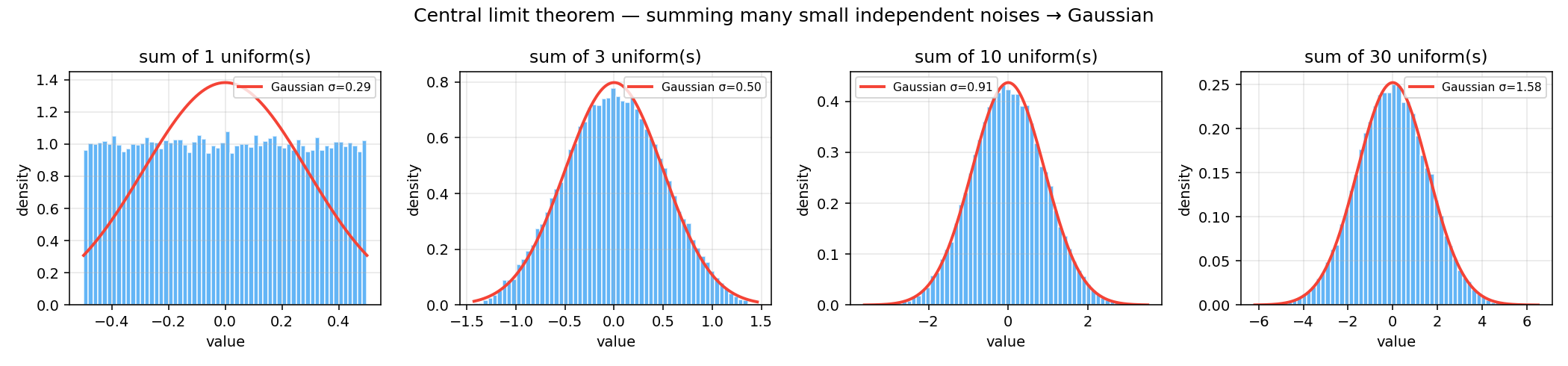
Part I detour: the full probability toolkit that makes this statement precise — Bernoulli → Binomial → Poisson → Normal → CLT — is built in Part I of this book. If your probability is rusty or if you want the derivations, read that first. If you trust the intuition above for now, continue.
The practical payoff arrives in Part I — Least Squares, where we build on this intuition to derive least-squares fitting as maximum likelihood under Gaussian noise — a rigorous justification for why so many algorithms in CV and ML use squared-error losses.
55. The Inverse Problem — Three Attacks¶
§2 introduced modelling and §3–§4 explained where noise comes from and why it tends to be Gaussian. Putting the two together gives the measurement model that underlies most of this book:
— a clean signal plus a random perturbation . The three “attacks” below are not three different ways of looking at the world. They are three different ways of building — three choices for how much structure you commit to before the data arrives.
Now we can state the general problem clearly.
Given noisy measurements , where is random with approximately known statistics. Goal: recover something useful about — specific values, the full function, or predictions at new inputs.
Three attacks exist. Each makes a different assumption about how much you already know about before you start.
Attack 1 — Averaging and signal processing¶
Premise: I can repeat the measurement at the same as many times as I want.
Take readings at a single . Their average has expected value (the noise averages out) and standard deviation . Double the readings → noise drops by . This is the famous rule — it is the whole reason that scientific instruments have “integration time” knobs.
Classical signal processing generalizes averaging — low-pass filtering, Wiener filtering, Kalman filtering — all are sophisticated forms of “combine many noisy observations to reduce uncertainty.”
Buys you: excellent estimates at the specific values you measured.
Doesn’t buy you: any predictions for new values.
Two flavours of averaging matter in practice:
| Ensemble average | Signal average (moving average) | |
|---|---|---|
| What you average | Many repeated trials at the same point | Neighbouring values across position or time |
| Assumption | Each trial has independent noise | Signal is locally smooth within the window |
| Practical limit | Need many repetitions of the same measurement | Blurs sharp edges and fine detail |
| Imaging example | Average 100 frames of the same scene | Slide a window across one frame, average pixels inside it |
In a lab you can often do ensemble averaging — hold everything still and repeat. In production imaging you rarely can (scene changes, one frame available), so signal averaging (spatial smoothing, Gaussian blur, moving average filter) is the practical tool. Wider window → more noise reduction but more blurring of real defect edges. Part II covers both in detail.
MVTec example: average multiple exposures of the same tile patch to suppress sensor noise, then apply a smoothing filter to separate the slow-varying background texture from sharp defect edges. This reduces noise and makes defect structure more visible — but only tells us about patches we have already imaged. It gives no prediction for unseen surfaces.
Parts II and III of this book develop this attack for the imaging case: sampling, sensors, pixels, contrast, and why raw-pixel operations run into fundamental limitations.
Attack 2 — Parametric fitting (known model form)¶
Premise: I already know the functional form of from physics or from prior knowledge. I just don’t know a handful of constants.
Examples:
Radioactive decay: — two unknowns .
Sensor calibration: — slope and offset.
Ideal gas: — fit to data.
Pick the constants that make the model best match the data. The standard criterion is least-squares: choose and to minimise the total squared gap between each measurement and the model’s prediction :
Intuitively: draw all possible lines through the scatter of points; the least-squares line is the one where the sum of the squared vertical distances from each point to the line is smallest. Squaring the gaps means large errors are penalised more heavily than small ones — a point twice as far from the line contributes four times the penalty. This is both a strength and a weakness: the fit responds strongly to every point, but a single outlier with a large gap pulls the line toward it to reduce that squared penalty. Least-squares is not outlier-robust.
The values of and that achieve this minimum can be computed exactly from the data — no iteration needed. This is what classical statistics calls regression. You’re not discovering what looks like; you’re nailing down a few numbers inside a form that was handed to you by domain knowledge. The full derivation — why squaring, why this specific formula, and its connection to maximum likelihood under Gaussian noise — arrives in Chapter 7.
Buys you: predictions at any , not just the measured ones.
Costs: if the assumed form is wrong, your predictions are wrong no matter how much data you collect.
MVTec example: the MVTec tile surfaces are flat and the lighting is fixed, so Lambert’s cosine law simplifies to — a linear relationship between true reflectance and pixel value . Fit (lamp gain) and (dark current) from a set of defect-free calibration patches using least-squares. Any patch whose pixel values deviate significantly from this fitted model is flagged as a defect. The model generalises across the whole surface — but only because the flat-surface, fixed-lighting assumption holds. Change the lamp angle or surface curvature and the calibration breaks.
Attack 3 — Flexible learning (machine learning)¶
Premise: I don’t know the form of . But I have many pairs and I’m willing to spend compute.
Pick a flexible hypothesis class — polynomials, kernels, neural networks, transformers — and find the member that best matches the data. You’re not committing to a specific form, just a space of forms. The algorithm chooses the form from the space.
Buys you: the ability to handle problems where no physical model exists — image classification, language, complex real-world mappings.
Costs: much more data, careful handling of overfitting, harder interpretation of the resulting model.
MVTec example: the Tile category contains five defect types — cracks, glue strips, gray strokes, oil spots, and rough patches — each with a different visual signature. No single parametric model covers all of them. Instead, train a CNN on the labeled MVTec patches: the network learns which combinations of local texture, edge, and contrast cues predict defective — without anyone specifying those cues explicitly. Attack 3 wins here because the variety of defect appearances is too complex to write down as a formula, but the patterns are learnable from data.
Parts V (CNNs) and VI (attention, vision transformers, multimodal models) of this book develop Attack 3. They are, structurally, elaborate parametric-fitting problems — but with hypothesis classes flexible enough to learn the form of rather than inherit it.
66. Three Attacks on the Same Data¶
To make the three attacks tangible, consider a simple simulation. We invent a true underlying function:
This is a mildly wavy curve — not a straight line, not wildly complicated. Think of it as the true reflectance profile of a surface as you slide a sensor across it. We then simulate 60 noisy measurements by sampling values uniformly between 0 and 6, computing the true at each, and adding Gaussian noise:
In a real experiment would be unknown. Here we keep it visible (dashed green line) so you can see how well each attack recovers it.
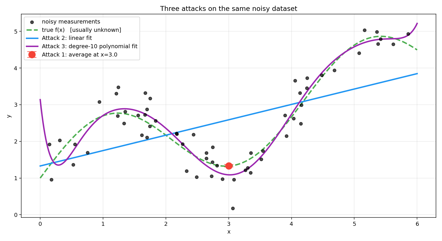
What the figure shows:
Attack 1 (red dot) — we pretend we can re-measure at many times and average those readings. The estimate lands very close to the true value at that one point, with a small error bar. But the rest of the curve is completely unknown to us — we have no way to predict at any other .
Attack 2 (blue line) — we fit a straight line through all 60 measurements. It predicts everywhere but misses the wiggle entirely. The assumed form (linear) is wrong, and no amount of extra data fixes a wrong assumption.
Attack 3 (purple curve) — we fit a degree-10 polynomial, which is flexible enough to track the wiggle. It follows the true curve closely in the middle, though it starts to stray at the edges where data is sparse. With even less data or a higher degree polynomial it would start fitting the noise bumps rather than the true signal — the failure mode called overfitting.
No attack is universally right. The skill is matching the attack to what you already know about your problem. In practice you often combine them — average noisy readings first (Attack 1), fit a calibration curve to the averages (Attack 2), then pass the calibrated data to a neural network (Attack 3).
The mathematics behind each attack is built up across the book — why averaging reduces error in Attack 1 (Part I, probability), how the slope is derived from data in Attack 2 (Chapter 7, maximum likelihood), and how overfitting is detected and controlled in Attack 3 (Chapter 12, training). Each concept is introduced only when the tools to explain it properly are in place.
77. From 1D Signals to Images to Multimodal AI¶
Everything above used a scalar input . Real problems are almost always higher-dimensional:
A pixel in an image — input is a 2D spatial coordinate, output is the intensity at that coordinate.
A full image — input is the image (a high-dimensional vector of pixels), output is a classification or a latent feature.
Video — input is an image indexed by time; noise and signal both have temporal structure.
Audio — input is a 1D signal over time; same framework, different dimensionality.
Multimodal — an input might contain an image and text and audio simultaneously; each modality is a different signal, and the task is to fuse them.
The mathematics scale cleanly: wherever we wrote for scalar , we can write for vector , or for vector output. The three attacks stay the same. Visualization gets harder, the amount of data needed grows (the curse of dimensionality), and the algorithms become heavier — but the problem statement doesn’t change.
This is why the book’s title is Signals to Transformers and not Pixels to Transformers: the framework subsumes pixels, tokens, audio, and video alike. A transformer processing a paragraph, a ViT processing an image, and a CLIP model fusing images with captions are all solving the same inverse problem — they just work in different signal spaces.
88. Signal Processing vs. Parametric Fitting vs. Machine Learning¶
The three attacks all start from the same data and the same goal — recover something useful about . What separates them is how much you assume about before you look at the data, and what you get back in return.
| Dimension | Attack 1 — Signal Processing | Attack 2 — Parametric Fitting | Attack 3 — Machine Learning |
|---|---|---|---|
| Prior assumption about | None about its form. Only that the signal is repeatable or locally smooth. | The functional form of is known from physics / domain knowledge. Only a few constants are unknown. | The form of is unknown. You only commit to a flexible hypothesis class (polynomials, kernels, neural nets). |
| What you choose | A filter / averaging window | A small set of parameters (e.g. ) | A hypothesis class + a learning algorithm |
| What you get back | A denoised estimate at the values you measured | An equation valid everywhere the assumed form holds | A learned function that maps any to a prediction |
| Generalises to new ? | No — only describes points you sampled | Yes — if the assumed form is correct | Yes — within the support of the training data |
| Data appetite | Modest: many readings at the same | Modest: few readings, but spread across | Large: many diverse pairs |
| Main failure mode | Over-smoothing destroys real edges / fine structure | Wrong functional form → systematically wrong predictions, no amount of data fixes it | Overfitting; poor extrapolation; opacity |
| What “fitting” means | Choosing kernel width, cutoff frequency | Solving for that minimises a loss (e.g. least-squares) | Solving for millions of weights that minimise a loss |
| Typical tools | Moving average, Gaussian blur, Wiener / Kalman filter, FFT | Linear regression, polynomial fit, exponential decay fit, calibration curves | CNNs, transformers, kernel methods, gradient boosting |
| Where taught | Signals & systems / DSP courses | Classical statistics / regression courses | ML / deep learning courses |
| MVTec tile example | Average frames + Gaussian blur to suppress sensor noise | Fit Lambert calibration; flag deviations as defects | Train a CNN on labelled defect patches across all five defect types |
How they relate¶
These are not three disjoint worlds — they sit on a spectrum of how much structure you bring to the problem:
What replaces the physics prior in ML?¶
A natural question: parametric fitting commits to a specific equation (, , etc.) handed down from physics. ML doesn’t. So what is its prior? It can’t be “anything goes” — that would never generalise.
The answer is that ML replaces the physics prior with a much weaker smoothness / regularity prior: nearby inputs should produce nearby outputs, shouldn’t wiggle wildly, the function should have some kind of structure that lets it be described by far fewer numbers than the training set contains.
Different ML models encode this weak prior in different ways:
| Model | Implicit prior on |
|---|---|
| Polynomial regression (degree ) | has bounded curvature up to order |
| Kernel methods (RBF, Gaussian process) | Nearby → nearby , controlled by a length-scale |
| CNN | Local patterns + translation invariance + hierarchical composition |
| Transformer | Long-range dependencies + permutation-equivariance over tokens |
| Neural net (generic) | Compositional smoothness — small change in usually means small change in |
So the contrast between Attack 2 and Attack 3 is really about where the information lives:
Attack 2 puts most of its information in the form. Physics tells you is a line, so all the data has to do is pin down two numbers. Tiny hypothesis class, little data needed — but if the form is wrong, the model fails silently no matter how much data you collect.
Attack 3 puts most of its information in the data. The hypothesis class is vast (millions of weights), and the only built-in prior is smoothness or structural symmetry. The data is what selects the actual shape of from that huge space — which is why ML is so data-hungry.
This is also why regularisation matters in ML but barely appears in parametric fitting: when your hypothesis class is small and physics-shaped, the form itself is the regulariser. When the class is huge, you need explicit pressure (weight decay, dropout, early stopping, data augmentation) to keep the model inside the smooth, well-behaved region of the space.
A few useful observations the table doesn’t show directly:
Attack 2 and Attack 3 share the same machinery. Both pick a hypothesis class and minimise a loss. Linear regression is just Attack 3 with a hypothesis class of size one (lines). A neural network is just Attack 2 with a hypothesis class wide enough to learn the form of . This is why linear regression appears in both statistics and ML courses — it is the bridge between them.
The boundary between Attack 1 and Attack 2 is not airtight. Kalman filtering, AR / ARMA modelling, and system identification are signal-processing methods that internally fit parameters of an assumed state-space or autoregressive model. The split here is pedagogical, not taxonomic — it keeps the three premises clearly separate for a learner.
In practice you chain them. Average noisy readings (A1), fit a calibration curve to the averages (A2), then feed the calibrated data into a neural network (A3). Real pipelines almost always combine all three.
9Summary¶
| Concept | Key idea |
|---|---|
| Measurement | — signal plus noise |
| Noise | Physical, statistical, typically Gaussian (CLT) |
| Inverse problem | Recover from pairs |
| Attack 1 | Average / filter at known values (signal processing) |
| Attack 2 | Fit parameters inside a known functional form (regression) |
| Attack 3 | Pick a flexible hypothesis class, let data choose the form (ML) |
| Three-attack split | By premise and output, not by which course teaches them |
| Signals | Pixels, tokens, audio, video — the same math covers all |
| Running example | MVTec AD Tile: filter/average (A1), fit Lambert calibration model (A2), train CNN on labeled patches (A3) |
Next → Part I — Math Foundations if you want the probability and linear algebra before the applied content, or skip to Part II — Signals and Measurement for the first applied chapter.